Reproducibility - Real Data Analysis • afpca

Overview

This vignette reproduces the real-data analysis from the paper “Functional Principal Components Analysis with Locally Adaptive Smoothing” using the afpca package. We apply Adaptive Functional Principal Components Analysis (Adaptive FPCA) to trial-averaged neural firing rate data recorded during a reaching task, and compare the results to the standard fpca.sc method from the refund package.

Setup

library(afpca)
library(refund)
require(tidyverse)
require(ggplot2)
require(tidyfun)
require(patchwork)

data(firing_rates_data)

Data

firing_rates_data contains trial-averaged mean activation profiles (spikes/sec) for 25 neurons over a 1.74-second window. Each row is one neuron, and the activation column stores its firing rate profile as a tfd functional data object. The time axis is shifted so that $t = 0$ corresponds to cue onset. These are the neuron-level averages displayed in Panel B1 of Figure 1 in the paper.

firing_rates_data |>
  tf_unnest(activation) |>
  mutate(activation_arg = activation_arg - 0.25) |>
  ggplot(aes(x = activation_arg, y = activation_value, group = neuron_no)) +
  geom_line(linewidth = 0.6, alpha = 0.5) +
  labs(x = "Time from cue (sec)", y = "Mean Activation (spikes / sec)") +
  theme_bw() +
  theme(text = element_text(size = 12))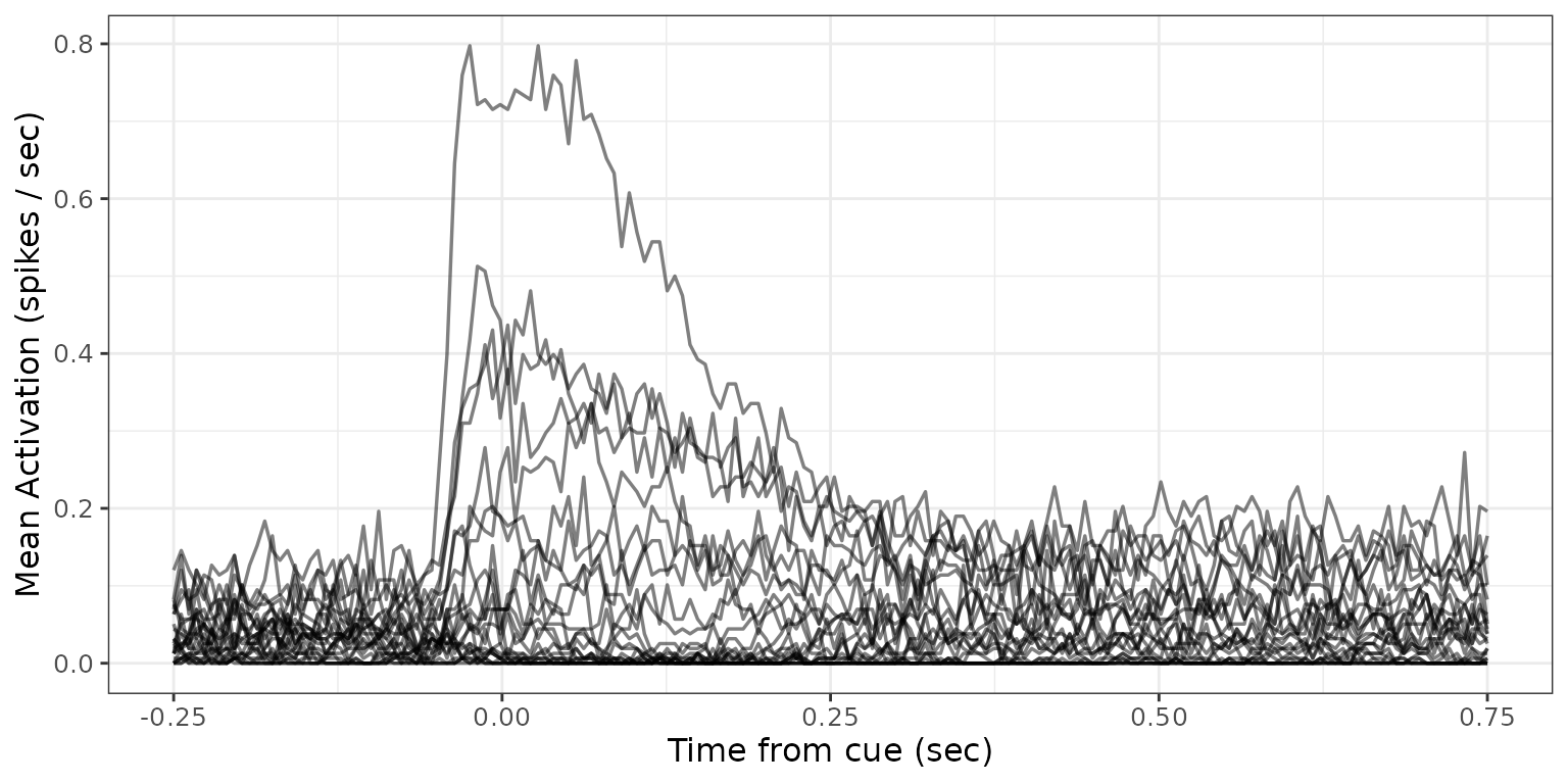

Figure 4

Figure 4 compares Adaptive FPCA against fpca.sc across two panels:

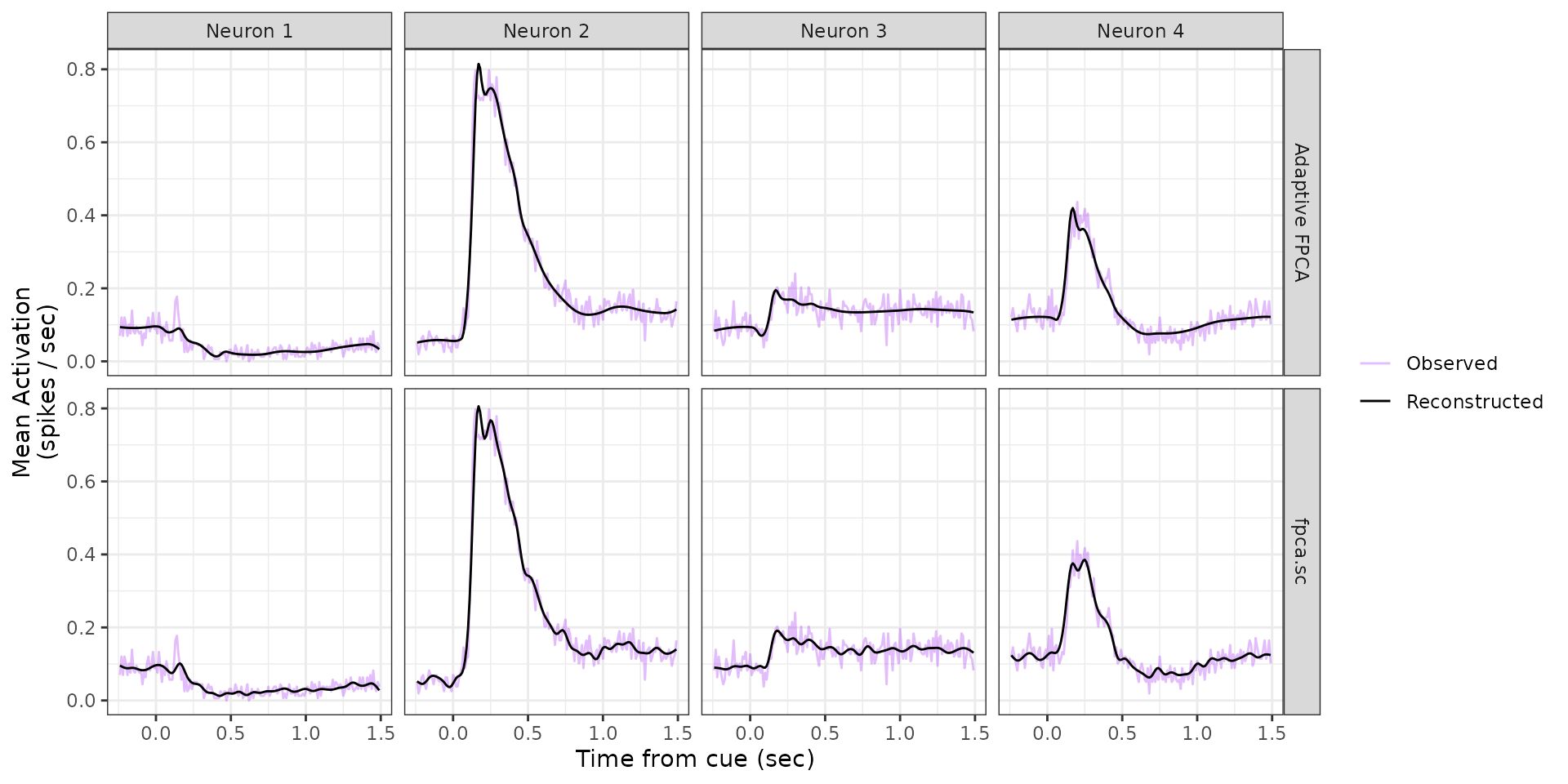
Panel A shows the first two estimated FPCs for each model, displayed as the estimated mean function (black) perturbed by the 25th (red) and 75th (blue) percentiles of the corresponding scores.
Panel B shows observed vs. reconstructed activation profiles for four representative neurons.

Model Fitting

We reshape the functional data into a numeric matrix (neurons × timepoints), fit both models, and flip FPC signs so the dominant pattern reflects increased post-cue activation.

Y.data <- firing_rates_data |>
  tf_spread(activation) |>
  select(-neuron_no) |>
  as.matrix()

# Adaptive FPCA
Fit.Adaptive.FPCA <- fpca.adapt(data = t(Y.data), nbs = 40, n.comp = 15)
Fit.Adaptive.FPCA$fpcs   <- Fit.Adaptive.FPCA$fpcs   * -1
Fit.Adaptive.FPCA$scores <- Fit.Adaptive.FPCA$scores * -1

# Standard FPCA
Fit.sc <- fpca.sc(Y = Y.data, nbasis = 40)
Fit.sc$efunctions <- Fit.sc$efunctions * -1
Fit.sc$scores     <- Fit.sc$scores     * -1

Panel A: Estimated FPC Patterns

The helper make_fpc_df() builds a tidy data frame for a single FPC, storing the mean and mean +/- FPC.

time_grid <- 1:174 / 100 - 0.25

make_fpc_df <- function(mu, phi, scores, fpc_no, model) {
  data.frame(
    Mu    = mu,
    plus  = mu + phi * quantile(scores, 0.75),
    minus = mu + phi * quantile(scores, 0.25),
    time  = time_grid,
    fpc_no = fpc_no,
    model  = model
  )
}

fpcs_data <- bind_rows(
  make_fpc_df(Fit.Adaptive.FPCA$mean, Fit.Adaptive.FPCA$fpcs[, 1],
              Fit.Adaptive.FPCA$scores[, 1], "Activation Pattern 1", "Adaptive FPCA"),
  make_fpc_df(Fit.Adaptive.FPCA$mean, Fit.Adaptive.FPCA$fpcs[, 2],
              Fit.Adaptive.FPCA$scores[, 2], "Activation Pattern 2", "Adaptive FPCA"),
  make_fpc_df(Fit.sc$mu, Fit.sc$efunctions[, 1],
              Fit.sc$scores[, 1], "Activation Pattern 1", "fpca.sc"),
  make_fpc_df(Fit.sc$mu, Fit.sc$efunctions[, 2],
              Fit.sc$scores[, 2], "Activation Pattern 2", "fpca.sc")
)

figure4_panelA <- fpcs_data |>
  ggplot(aes(x = time)) +
  geom_line(aes(y = Mu),    colour = "black") +
  geom_line(aes(y = plus),  colour = "blue") +
  geom_line(aes(y = minus), colour = "red") +
  facet_grid(model ~ fpc_no) +
  labs(x = "Time from cue (sec)", y = "Mean Activation\n(spikes / sec)") +
  theme_bw() +
  theme(text = element_text(size = 11))

figure4_panelA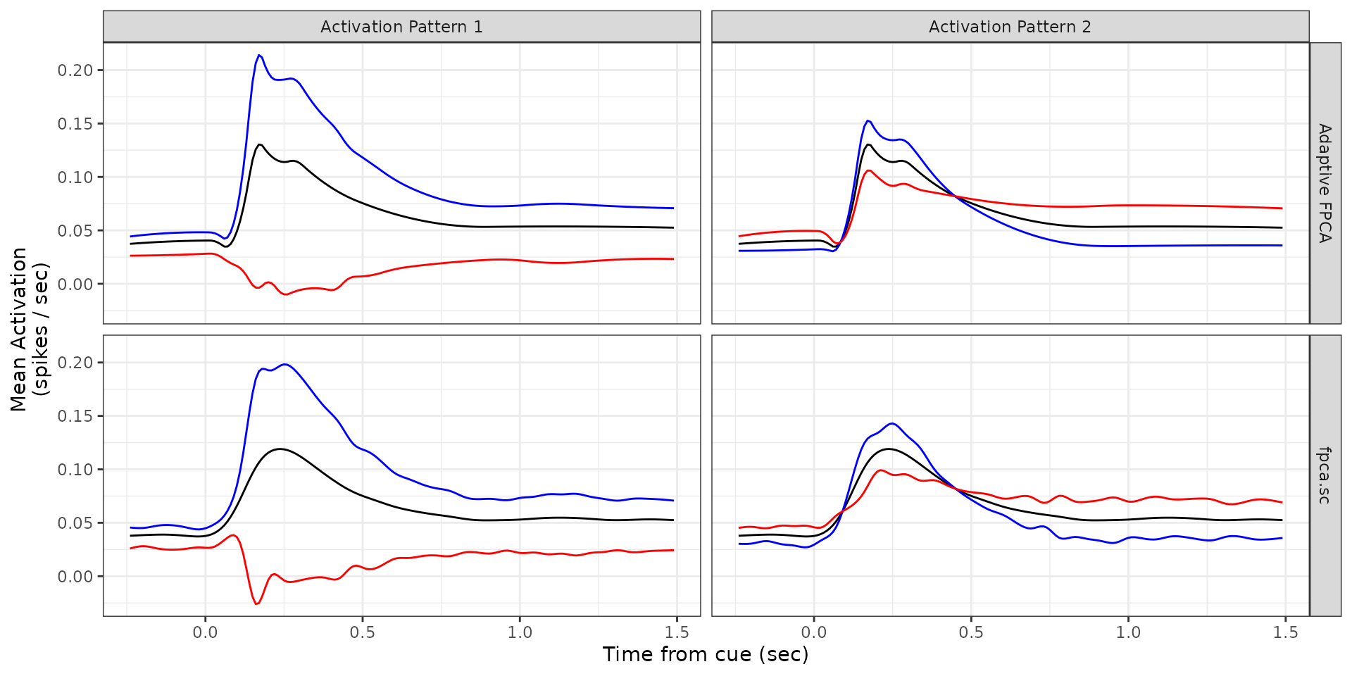

Panel B: Observed vs. Reconstructed

The helper make_neuron_df() pairs observed and model-reconstructed profiles for a single neuron. We do this for four representative neurons under each model.

make_neuron_df <- function(idx, label, model_name, observed_mat, fitted_mat) {
  data.frame(
    observed = observed_mat[, idx],
    fitted   = fitted_mat[, idx],
    time     = time_grid,
    model    = model_name,
    neuron   = label
  )
}

neuron_idx    <- c(1, 4, 15, 25)
neuron_labels <- paste("Neuron", 1:4)

neurons_data <- bind_rows(
  Map(make_neuron_df, neuron_idx, neuron_labels,
      "Adaptive FPCA", list(t(Y.data)), list(Fit.Adaptive.FPCA$Y_hat)),
  Map(make_neuron_df, neuron_idx, neuron_labels,
      "fpca.sc",       list(t(Y.data)), list(t(Fit.sc$Yhat)))
) |> bind_rows()

figure4_panelB <- neurons_data |>
  ggplot(aes(x = time)) +
  geom_line(aes(y = observed, colour = "Observed"),      alpha = 0.3) +
  geom_line(aes(y = fitted,   colour = "Reconstructed")) +
  facet_grid(model ~ neuron) +
  labs(x = "Time from cue (sec)", y = "Mean Activation\n(spikes / sec)") +
  scale_color_manual(values = c("Observed" = "purple", "Reconstructed" = "black")) +
  theme_bw() +
  theme(text = element_text(size = 11), legend.title = element_blank())

figure4_panelB